Tutorial_STMSC (Example with DLPFC Data)

Before running the model, please download the input data via: https://drive.google.com/drive/folders/1EzLhPeMaMA02fmZquNYwixMK0MSe7UAA?usp=drive_link

1. Environment Setup

import os
import sys
import random
import warnings
import numpy as np
import pandas as pd
from pandas import Categorical
import torch
from sklearn.mixture import GaussianMixture
from sklearn.metrics import pairwise_distances, adjusted_rand_score, normalized_mutual_info_score
import scanpy as sc
import cv2
from STMSC import utils,train,load_data_preprocess

warnings.filterwarnings("ignore")
device = torch.device('cuda:0')

2. Load and Preprocess Data

Using STMSC with Your Own Dataset

This notebook demonstrates how to run STMSC on your own dataset. To ensure compatibility, your input data should meet the following minimum requirements.

📋 Required Data Format for Running STMSC

Data Type	Variable Name	Data Location	Field	Description
ST data(spots × genes)	adata_st_list_raw(e.g., [adata_st1, adata_st2, ...])	adata_st.obs	['slice_id']	Slice identifier
			['x_pixel'], ['y_pixel']	Spatial coordinates (in image pixels)
			['layer'] (optional)	Ground-truth domain label
		adata_st.var	var_names	Gene symbols
	adata_img_list_raw(e.g., [img1, img2, ...])	.tif images	—	Histology image of each tissue slice
scRNA-seq data(cells × genes)	adata_ref	adata_ref.obs	['celltype']	Cell type for each cell
		adata_ref.var	var_names	Gene symbols (must match ST data)

For Example

# spatial data
# slice_idx = [151507, 151508, 151509, 151510]
# slice_idx = [151669, 151670, 151671, 151672]
slice_idx = [151673, 151674, 151675, 151676]

anno_df = pd.read_csv('LIBD/barcode_level_layer_map.tsv', sep='\t', header=None)

adata_st1 = sc.read_visium(path="LIBD/%d" % slice_idx[0],
                        count_file="%d_filtered_feature_bc_matrix.h5" % slice_idx[0])
spatial1=pd.read_csv(os.path.join('LIBD', str(slice_idx[0]), "spatial/tissue_positions_list.txt"),sep=",",header=None,na_filter=False,index_col=0)
anno_df1 = anno_df.iloc[anno_df[1].values.astype(str) == str(slice_idx[0])]
anno_df1.columns = ["barcode", "slice_id", "layer"]
anno_df1.index = anno_df1['barcode']
adata_st1.obs = adata_st1.obs.join(anno_df1, how="left")
adata_st1.obs["x_pixel"]=spatial1[4]
adata_st1.obs["y_pixel"]=spatial1[5]
adata_st1 = adata_st1[adata_st1.obs['layer'].notna()]


adata_st2 = sc.read_visium(path="LIBD/%d" % slice_idx[1],
                        count_file="%d_filtered_feature_bc_matrix.h5" % slice_idx[1])
spatial2=pd.read_csv(os.path.join('LIBD', str(slice_idx[1]), "spatial/tissue_positions_list.txt"),sep=",",header=None,na_filter=False,index_col=0)
anno_df2 = anno_df.iloc[anno_df[1].values.astype(str) == str(slice_idx[1])]
anno_df2.columns = ["barcode", "slice_id", "layer"]
anno_df2.index = anno_df2['barcode']
adata_st2.obs = adata_st2.obs.join(anno_df2, how="left")
adata_st2.obs["x_pixel"]=spatial2[4]
adata_st2.obs["y_pixel"]=spatial2[5]
adata_st2 = adata_st2[adata_st2.obs['layer'].notna()]

adata_st3 = sc.read_visium(path="LIBD/%d" % slice_idx[2],
                        count_file="%d_filtered_feature_bc_matrix.h5" % slice_idx[2])
spatial3=pd.read_csv(os.path.join('LIBD', str(slice_idx[2]), "spatial/tissue_positions_list.txt"),sep=",",header=None,na_filter=False,index_col=0)
anno_df3 = anno_df.iloc[anno_df[1].values.astype(str) == str(slice_idx[2])]
anno_df3.columns = ["barcode", "slice_id", "layer"]
anno_df3.index = anno_df3['barcode']
adata_st3.obs = adata_st3.obs.join(anno_df3, how="left")
adata_st3.obs["x_pixel"]=spatial3[4]
adata_st3.obs["y_pixel"]=spatial3[5]
adata_st3 = adata_st3[adata_st3.obs['layer'].notna()]

adata_st4 = sc.read_visium(path="LIBD/%d" % slice_idx[3],
                        count_file="%d_filtered_feature_bc_matrix.h5" % slice_idx[3])
spatial4=pd.read_csv(os.path.join('LIBD', str(slice_idx[3]), "spatial/tissue_positions_list.txt"),sep=",",header=None,na_filter=False,index_col=0)
anno_df4 = anno_df.iloc[anno_df[1].values.astype(str) == str(slice_idx[3])]
anno_df4.columns = ["barcode", "slice_id", "layer"]
anno_df4.index = anno_df4['barcode']
adata_st4.obs = adata_st4.obs.join(anno_df4, how="left")
adata_st4.obs["x_pixel"]=spatial3[4]
adata_st4.obs["y_pixel"]=spatial3[5]
adata_st4 = adata_st4[adata_st4.obs['layer'].notna()]

adata_st_list_raw = [adata_st1, adata_st2, adata_st3, adata_st4]
#Read in hitology image
img1=cv2.imread(os.path.join('LIBD/', str(slice_idx[0]), str(slice_idx[0])+"_full_image.tif"))
img2=cv2.imread(os.path.join('LIBD/', str(slice_idx[1]), str(slice_idx[1])+"_full_image.tif"))
img3=cv2.imread(os.path.join('LIBD/', str(slice_idx[2]), str(slice_idx[2])+"_full_image.tif"))
img4=cv2.imread(os.path.join('LIBD/', str(slice_idx[3]), str(slice_idx[3])+"_full_image.tif"))
adata_img_list_raw = [img1, img2, img3, img4]

load_data_preprocess.extract_histology_features(adata_st_list_raw, adata_img_list_raw)
utils.set_seed(2024)
adata_st_list = load_data_preprocess.align_spots(adata_st_list_raw, plot=False)
adata_ref = sc.read_h5ad('LIBD/human_MTG_snrna_norm_by_exon.h5ad')
adata_ref.obs['celltype'] = adata_ref.obs['cluster_label']
adata_st, adata_basis, _ = load_data_preprocess.preprocess(
    adata_st_list, adata_ref,
    sample_col=None,
    n_hvg_group=500
)
adata_st_list = load_data_preprocess.align_spots_3D(adata_st_list_raw)
adata_st.obsm['spatial_aligned'] = np.vstack([np.array(lst) for a in adata_st_list for lst in a.obsm['spatial_aligned']])

Using the Iterative Closest Point algorithm for alignemnt.
Detecting edges...
Aligning edges...
Finding highly variable genes...
8062 highly variable genes selected.
Calculate basis for deconvolution...
Preprocess ST data...
Start building a graph...
Radius for graph connection is 150.7000.
9.8415 neighbors per cell on average.
Using the Iterative Closest Point algorithm for alignment.
Detecting edges...
Aligning edges...

3.Learn map matrix

🔄 Customizing the Deconvolution Step

STMSC is designed to be modular and flexible. We encourage users to adopt the most appropriate deconvolution strategy based on the characteristics of their own data. If you prefer to use an alternative method (e.g., RCTD, Tangram, or your own approach) to compute a mapping matrix, you can seamlessly integrate it into the STMSC.

✅ How to Use a Custom Mapping Matrix

1. Compute your deconvolution result using any external method.

2. Save the resulting mapping matrix as a .npy file.

3. In the STMSC, simply specify the file path as:map_path = “my_map_matrix.npy”

map = train.learn_mapping_matrix(adata_st, adata_basis, lam=7, epoch=5000)
np.save('map_673_lam_7.npy', map)

100%|██████████| 5000/5000 [1:51:14<00:00,  1.33s/it]

4. Spatial Graph Construction

adata_st.obsm["graph"] = utils.construct_combined_graph(
    adata_st=adata_st,
    loc_3D=adata_st.obsm['spatial_aligned'],
    map_path='map_673_lam_7.npy',
    bl=0.1,
    bll=0.1
)

5. Train STMSC Model

model, latent = train.train_stmsc_model(adata_st, adata_basis, device=device,epochs=5000)

100%|██████████| 5000/5000 [12:06<00:00,  6.88it/s]

6. Domain Identification

gm = GaussianMixture(n_components=7, covariance_type='tied', init_params='kmeans')
pred_labels = gm.fit_predict(latent)
pred_labels = Categorical(pred_labels)

splits = [a.shape[0] for a in adata_st_list_raw]
idxs = np.cumsum([0] + splits)
for i in range(4):
    true = adata_st_list_raw[i].obs['layer']
    pred = pred_labels[idxs[i]:idxs[i+1]]
    print(f'Slice {i}, ARI = {adjusted_rand_score(true, pred):.4f}, NMI = {normalized_mutual_info_score(true, pred):.4f}')

print(f'Total ARI = {adjusted_rand_score(adata_st.obs["layer"], pred_labels):.4f}')
print(f'Total NMI = {normalized_mutual_info_score(adata_st.obs["layer"], pred_labels):.4f}')

Slice 0, ARI = 0.5749, NMI = 0.7121
Slice 1, ARI = 0.6319, NMI = 0.7458
Slice 2, ARI = 0.5611, NMI = 0.7047
Slice 3, ARI = 0.5998, NMI = 0.7156
Total ARI = 0.5875
Total NMI = 0.7076

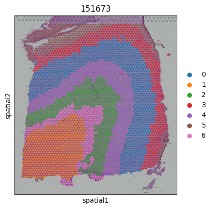
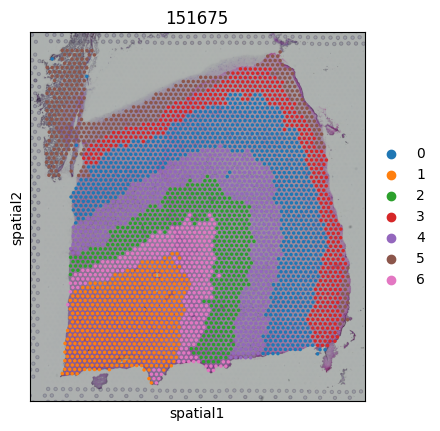
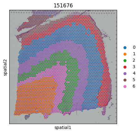
7. Visualization

for i,adata_sub in enumerate(adata_st_list):
    pred = pred_labels[idxs[i]:idxs[i+1]]
    adata_sub.obs['Region'] = pred
    sc.pl.spatial(adata_sub,color=["Region"],title=str(slice_idx[i]))